Math 223, Linear Algebra

These notes are based on lectures given by Professor Mikäel Pichot for MATH 223, Linear Algebra at McGill University during the Winter 2024 semester.

Chapter 1: Vectors in and , Spatial Vectors

Complex Numbers

The following are some of the standard sets of numbers.

• Natural numbers: (for the purposes of this class, )
• Integers:
• Rational numbers:
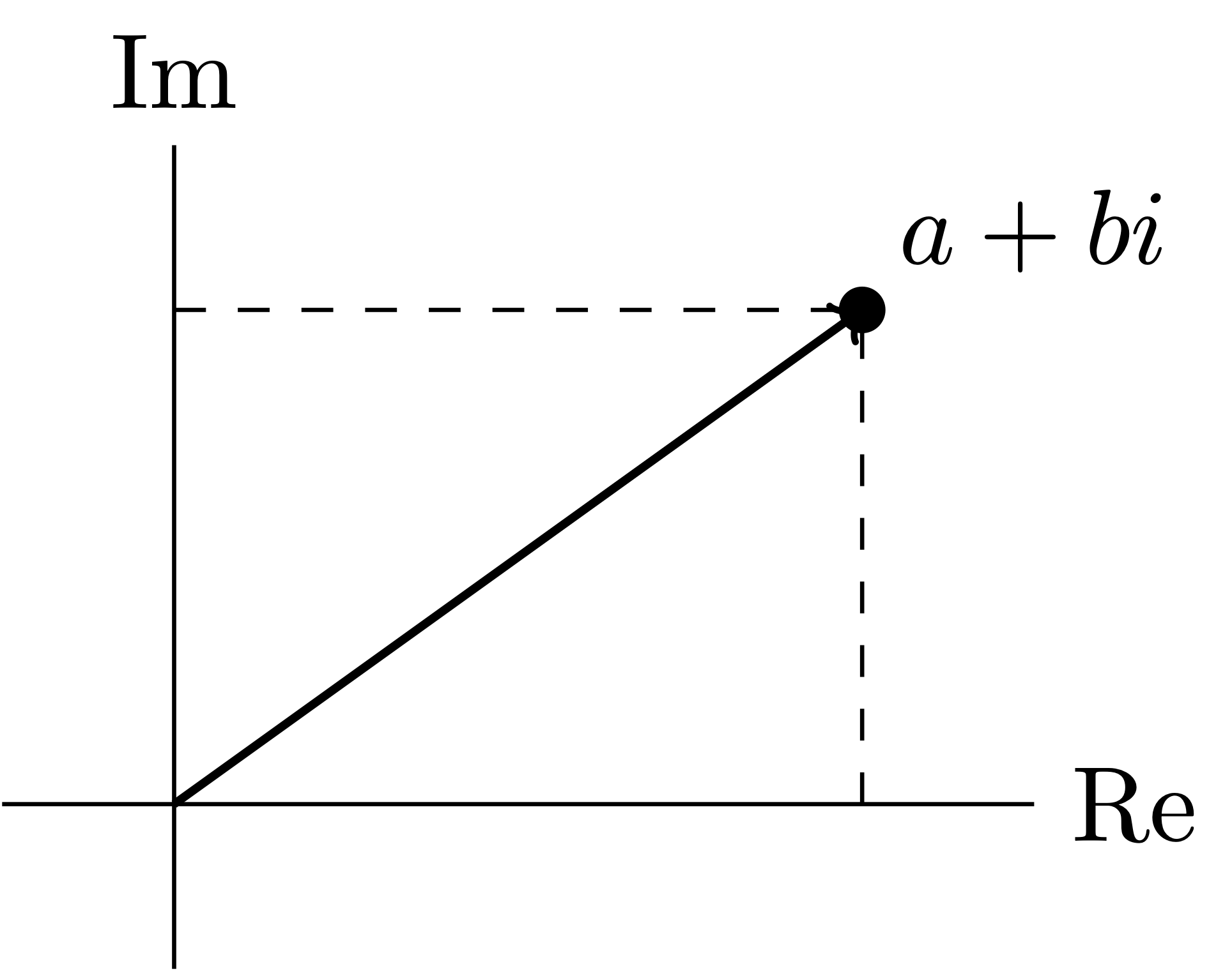
• Real numbers: is the set of all numbers on the real number line including both rational and irrational numbers.
• Complex numbers: ( is called the real part and is called the imaginary part).

These standard sets can be arranged in increasing order:

Definition (Imaginary Unit)

is the imaginary solution to

Theorem

In , is not defined.

Unlike real numbers which are represented on a number line, complex numbers are represented on the complex plane where the -axis is the axis while the -axis is the axis. Notice the connection made with a vector .

Theorem

We need complex numbers in order to be able to solve all non-constant polynomials ().

Definition (Root/Solution)

A root/solution, , of a polynomial, , is .

Theorem

Every non-constant polynomial has a solution in .

Corollary

In , every polynomial can be factored. Furthermore, by repeated factoring, we can get linear factors which are the roots of the polynomial.

Operations with Complex Numbers

We also want to define operations between where and . The result of these operations should also be in .

• Equality of Complex Numbers: Two complex numbers and are considered equal if and only if and .
• Addition of Complex Numbers:
• Multiplication of Complex Numbers: To define multiplication, observe the identity .
• Complex Conjugate:
  Geometrically, this is represented by a reflection over the real axis of the complex plane
• Inverses of Complex Numbers:

Theorem

Corollary

Proof.
First, we prove the forward implication: .

Secondly, we prove the converse: .

QED

Theorem

The inverse of a complex number is a complex number.

Proof.

QED

Lemma

Definition (Euclidean Norm/Modulus of a Complex Number)

From the geometric representation of a complex number, we can find the magnitude of the vector using .

Theorem

Proof.

1. Show
2. Show

QED

Standard Algebraic Structures

Let be a “set with multiplication” (i.e., the multiplication operation is defined on elements in the set and the product is also in that set).

Definition (Multiplicative Inverse)

Given , we say is an inverse of if . Furthermore, we say that is invertible if such that is an inverse of .

Example: The inverse of is . However, 2 is not invertible in or .

Lemma

If an inverse of exists, it is unique.

A matrix is invertible if s.t. .

A note about notation:

Definition (Ring)

A nonempty set is a ring if addition and multiplication is defined on the set and respects the following axioms:

• Associativity: and
• Zero element:
• Negative:
• Commutative addition:
• Distributive:

A ring can be called a commutative ring if .

Thus, are rings while is not a ring.

Definition (Field)

A field is a commutative ring if every nonzero has a multiplicative inverse (i.e., ).

Thus, although is a ring, it is not a field because some elements do not have a multiplicative inverse (e.g., integers ). are fields.

Fields are the building blocks of vector spaces. In this course, we will focus on fields and .

Example: Prove that is not invertible.

Proof.
By contradiction, assume is invertible.

Since this is a contradiction, must be not invertible.
QED

Geometry of Complex Numbers

Since complex numbers can be represented on the complex plane, we can examine the geometry of complex numbers.

Example: A circle of radius can be represented by the following set of points:

If we look at the unit circle, we can notice the periodicity of : The implication of this is that it is very easy to take to large exponents since .

Euler’s Formula

Euler’s formula established a relationship between trigonometric functions and the complex exponential function.

If we observe that , we can conclude that must parametrize the unit circle.

Chapter 2: Algebra of Matrices

A matrix over a field is a rectangular matrix of the form:

The element is the entry in row and column . A matrix with rows and columns is called an matrix.

Matrix Addition and Scalar Multiplication

Matrix Addition is defined as follows:

Matrix Scalar Multiplication is defined as follows:

Matrix Multiplication

Matrix multiplication is defined between a matrix with dimensions and a matrix with dimensions whose product is a matrix. Note that matrix multiplication is not commutative.

Matrix multiplication is described by the equation below where the element is the dot product of row in and column in .

Given square matrices and , each element in the product is defined by the following sum.

Transpose of a Matrix

The transpose of a matrix denoted is the matrix obtained by making the columns in into rows in .

Square Matrices

Definition (Square Matrix): A square matrix has the same number of rows and columns (i.e., it is an matrix).

Definition (Diagonal): The diagonal of a square matrix are the entries .

Definition (Trace): The trace of , denoted is the sum of the diagonal elements.

Definition (Identity Matrix)

The identity matrix, denoted is the -square matrix with 1’s in the diagonal and 0’s everywhere else. A unique property is that for any matrix , .

Chapter 4: Vector Spaces

In a vector space where is the field of scalars, we can define vector addition and scalar multiplication as follows:

Definition (Vector addition and Scalar Multiplication)

• Vector addition: For any , we assign a sum .
• Scalar multiplication: For any and , we assign a product .

In addition to defining vector addition and scalar multiplication on a nonempty set, the following axioms must hold for arbitrary vectors in a vector space .

• Associative vector addition:
• Origin/zero vector or neutral element for addition:
• Negative:
• Commutative:
• Distributive scalar: where
• Distributive vector: where
• Associative scalar multiplication:
• Unit scalar: where

Definition (Vector Space)

A vector space is a nonempty set with vector addition and scalar multiplication defined and respects all of the above axioms.

Examples of Vector Spaces

Space

Given an arbitrary field , the notation is used to denote the set of all -tuples of elements in .

In , vector addition is defined as: .

In , scalar multiplication is defined as: .

Polynomial Space

Let denote the set of all polynomials of the form where .

The degree of a polynomial refers to the highest power in the polynomial with a nonzero coefficient. Exceptionally, the degree of the zero polynomial is undefined.

Here, vector addition and scalar multiplication can be represented by adding polynomials and multiplying each term of the polynomial by the scalar respectively.

The standard basis of this space is: .

The set of all polynomials is denoted . Therefore, if .

Also, although polynomials have multiplication defined, they are only well defined in since but .

Matrix Space

is the set of all matrices with fields in . We can use the matrix addition and scalar multiplication of matrices.

Multiplication is well defined on square matrices in vector space since the product of two matrices is still .

The standard basis of is:

Function Space

is the set of all functions with nonempty domain set into a field . We can denote this using set builder notation as . This function assigns a value in .

Vector addition of two functions and in is the function .

Scalar multiplication of a function in and in is the function .

The zero vector in is called the zero function and maps every values to the zero element (i.e., ).

A function in can be entirely defined by an -tuple where is the size of . For example, if , then a function .

Kronecker functions indexed by can be used to define the standard basis of .

Linear Combinations and Spanning Sets

Definition (Linear Combination)

A vector is a linear combination of a finite set of vectors if there exists which satisfy .

Example: Express as a linear combination of . We can solve using the following augmented matrix and row reducing.

After solving, we find that .

What happens if we get an inconsistent solution? This would suggest that the vector is not in the span of the other vectors and it is linearly independent from them.

Definition (Spanning Set)

If every vector in a vector space can be expressed as a linear combination of vectors , then we can say . In other words, the span of the set of vectors is the set of all linear combinations those vectors.

The canonical basis vectors can be used to span or .

The following example illustrates how spans over contrasts but is connected to spans over .

Example: Let and be the standard basis of .

This example shows that while can be spanned by just 2 vectors, we need 4 vectors to span it over . It can be shown that in general can be spanned in vectors over and vectors over .

Remark. The properties of spans over fields, like many theorems over fields, do not hold in a generalization to rings. Spans over rings are studied in a different field (pun totally intended) of study and are more involved.

Subspaces

Definition (Subspace)

If is a subset of a vector space over a field and is a vector space over with respect to the vector addition and scalar multiplication operations on , then is a subspace of .

In order to show that a set is a vector space, normally, we would need to show that it satisfies the eight axioms outlined previously. However, if is the subset of a known vector space , some of the axioms automatically hold so we do not need to reprove them.

Theorem (Subspace Criterion)

If is a subset of a known vector space , we can use the subspace criterion to prove that is also a vector space. is subspace of if and only if:

1. Zero vector:
2. Closed under vector addition:
3. Closed under scalar multiplication:

The last two properties can be combined to form the equivalent property which says that the linear combination of is also in . This fact can be used to show that the span of some vectors in a vector space forms a subspace. Also, notice that closed under scalar multiplication implies the existence of the zero vector since we can argue that .

Proposition

There are only 2 subspaces of itself (where or ).

Proof. The subspaces of are .

is always a subspace and it is the smallest subspace since all vector spaces contain the zero vector. This also means that we cannot have an empty subspace.

is also obviously a subspace since and is a vector space.

Now, we prove that there is no other subset of . Let be a subspace of . We know that or . We need to show that if .

Let s.t. .
which means that the other subset must be all of .

Spanning sets can be shown to be subspaces. The proof by the subspace criterion is quite trivial since it is analogous to linear combinations. However, it shows that for any subspace we can find a set of vectors which spans it.

Proposition

The is a subspace of . This can be trivially proven by the subspace criterion.

Intersections, sums, and direct sums

Let and be subspaces in some vector space over the field .

Intersections

Proposition

The intersection is a subspace.

Proof.
Let ,

(a) Closed under vector addition
and > > and

Since is a subspace, .
Since is a subspace,
Therefore, .

(b) Closed under scalar multiplication

Since and are subspaces, they are closed under scalar multiplication so and .
Therefore, .

QED

Unions

Proposition

The union is a subspace if and only if or .

Proof.
(a) Forward implication
Assume is a subspace.
For proof by contradiction, assume and .
.

Since and , . This violates the subspace criterion which is a contradiction.

(b) Converse
If then .
If then .
Since and are both subspaces, in all cases, is a subspace.

QED

Sums

Proposition

The sum is a subspace.

Proof.
Let , , and . Then, .

(a) Closed under vector addition
> > and > >

(b) Closed under scalar multiplication
> > and since and are closed under scalar multiplication.

QED

Corollary

Proof.
(a)
Suppose and . Then, .
By definition, the vector is a linear combination of a vector from and a vector from so it is in .

(b)
Let . By definition, where , and .
and , so

QED

Direct Sums

Definition (Direct Sum)

A sum is a direction sum, denoted , if .

Proposition

and are in direct sum a non-zero vector has a unique decomposition (i.e., and are unique).

Proof.
(a) Forwards implication
If and are in direct sum, then .
Assume for contradiction where and .
> > > > and
Therefore, which only contains the zero vector, so . This is a contradiction.

(b) Converse
A non-zero vector has a unique decomposition and are in direct sum.
Contrapositive: and are not in direct sum does not have a unique decomposition.
and are not in direct sum means .
So, we can rewrite as and since and , this is a different but still a valid decomposition of .

QED

How to span a vector space

Building a spanning set

We can inductively build a spanning set of a vector space. Let be a vector space over .

Base case: the smallest possible vector space is .

Inductive step: If , halt. Otherwise, so we take a vector . We add the span of this vector to such that .

As long as , there always exists a vector . In the end, we find vectors such that .

This iterative process only halts after steps if and only if the vector space is finite dimensional with dimension . The choice of vector in each inductive step does not matter as long as it is not already in before it is added.

Dimension

Definition (Finite Dimensional Space)

A vector space is finite dimensional if it can be spanned by finitely many vectors. (i.e., such that ). If it cannot be spanned by finitely many vectors, it is infinite dimensional.

Definition (Dimension)

is the smallest number of vectors that span . Special cases, if , then and if is infinite dimensional, then .

Example: is a finite dimensional space spanned by its standard basis vectors .

Example: Show that .

Proof.

For contradiction, assume is spanned by finitely many polynomials: . There exists one polynomial in this set that has the highest degree. Let that polynomial be with . Then all polynomials with degree greater than cannot be in the span of these polynomials since vector addition and scalar multiplication as defined on polynomials does not increase the max degree. Therefore, must be infinite dimensional.

QED

Linear Independence

Definition (Linear Independence)

A set of vectors are linearly independent if

where .

Given vectors , to determine if they are linearly independent, we solve the system (using Gaussian Elimination). If the solution set is only the zero vector, then . Otherwise, there exists a non-trivial solution and the set of vectors are linearly dependent.

Definition (Linear Dependence)

Naturally, a set of vectors are linearly dependent if they are not linearly independent. i.e.,

Proposition

A set of vectors are linearly dependent if and only if there exists one of the vectors is in the span of the rest of the vectors.

Proposition

If the determinant of an upper triangular matrix (computed by multiplying the entries along the diagonal) is zero if and only if the columns of the matrix are linearly dependent.

Main Basis Theorem

Definition (Basis)

The basis of a vector space is a set of vectors that are linearly independent and a spanning set of .

Although the notions of spanning sets and linearly independent sets doesn’t really care about the ordering of the vectors, it is often helpful to express a basis as a tuple so that the basis vectors can be used for a coordinate system.

Lemma

The number of vectors in the basis of is equal to .

Proof.

Let be a basis of .
Since the set is linearly independent, .
Since the set is spanning, .
Putting this together, .

QED

Of course, this means that given two bases , then .

Often when we want to determine if a set of vectors forms a basis of a vector space, the number of vectors is equal to the dimension. If it is not, we can immediately determine that it is not due to the previous Lemma (if there are fewer vectors it won’t be a spanning set while if there are more vectors it won’t be a linearly independent set). However, when the number of vectors matches the dimension, it is redundant to check both spanning and linear independence, since they imply each other.

Proof.

Given .

If is spanning, then it must also be minimally spanning since any fewer vectors cannot span all of .
If is linearly independent, it must also be maximally linearly independent since any more vectors in will be in .
Thus, if either condition is met, then is a basis.

In practice, it is often easier to prove linearly independent rather than spanning.

Theorem (Basis Theorem)

A basis is the minimal spanning set and the maximal linearly independent set. (n.b., although this does not imply bases are unique, it does imply that all bases of the same vector space have the same cardinality).

It is also often helpful to have a standard basis for vectors spaces. The standard bases and their respective dimensions are:

1. Space (dimension )
   
2. Space (dimension )
   
3. Space (dimension )
   
4. Space where is finite (dimension )
   

Coordinates

Theorem (Basis-Coordinates)

is a basis of if and only if every vector can be expressed as a unique linear combination of the basis vectors.

Proof.

(a) Forwards implication

It is trivial to prove that can be expressed as a linear combination of the basis vectors since the basis vectors are a spanning set of .

We will prove uniqueness by contradiction. Assume for contradiction, that there are two coordinates and .
So, .
By subtraction, we find that . Since is linearly independent, and so . This is shows that the two coordinates must have been identical to begin with thus proving uniqueness. (Note the connection with the proof of unique decomposition for )

(b) Converse

Once again, it is trivial to show that if every as unique coordinates, then is a spanning set of .

To prove linear independence, we need to show that the only solution to is the trivial solution. And, indeed it is, because vectors have unique coordinates, . Thus, we have shows that is also linearly independent.

Since is both a spanning set of and linearly independent, it is a basis of .

QED

Example: Consider the standard basis of and a vector .

It can be expressed as the following sum:

To find the coordinates of a vector in an alternative basis, solve the following linear system:

Example: Let and consider the function space . Find the coordinates of in the standard basis.

Finding a basis

Basis Algorithm

Let . The basis algorithm can be used to get a basis of .

1. Define matrix where the rows correspond to the vectors.

2. Use Gaussian Elimination to get Row Echelon Form, matrix .

3. The non-zero rows in form a basis of .

Proof of correctness.

The elementary row operations do not affect the row space of the matrix, it is an invariant (row space is the span of the row vectors).
When we get to an REF, the vectors are linearly independent.
So the non-zero vectors in are linearly independent and still form a spanning set of . This is the definition of a basis of .

More Basis Theorems

Theorem (Transfer theorem)

If is a spanning set of and is a linearly independent set in , then both and and are bases of .

Theorem (Basis extraction theorem)

If , then some subset forms a basis of .

Casting-Out Algorithm

We can use the basis extraction theorem to actually extract a basis from a spanning set.
Like the basis algorithm, let . The casting-out algorithm will extract a basis of from .

1. Define matrix where the columns correspond to the vectors.

2. Use Gaussian Elimination to get Row Echelon Form, matrix .

3. The original vectors corresponding to the columns with the pivots in for a basis of .

Proof of correctness.
The linear dependency relations between columns are preserved by elementary operations.

Theorem (Basis extension theorem)

Given a linearly independent set in . There exists in such that forms a basis of .

Corollary

If is a subspace of , then .

Corollary

If is a subspace of , there exists a subspace called a supplement of such that .

Note that supplements are not unique. Example, in , all lines not on a plane are valid supplements. The supplement are the vectors added in the Basis Extension Theorem.

Theorem (Basis juxtaposition theorem)

Suppose that and are two subspaces in direct sum (i.e., ). Let be a basis of and be a basis of . Then, is a basis of .

Corollary

Chapter 5 and 6: Linear Mappings and Matrices

A platter of definitions

Definition (Transformation)

A transformation (also referred to as map or function) takes an element and assigns a value , denoted . The set is called the domain and the set is called the co-domain of .

Definition (Injective)

A transformation is injective if . The equivalent contrapositive is .

Connection to calculus: the horizontal line test.

Definition (Surjective)

A transformation is surjective if .

Connection to calculus: range of the function is the codomain.

Definition (Bijective)

A transformation is bijective if it is both injective and surjective.

Definition (Invertible)

A transformation is invertible if there exists such that and .

Lemma

Let and be transformations.

Proof.

We assume but for contradiction assume not injective or not surjective.

If not injective, where such that .
Then apply to both sides to get .
Since , which is a contradiction and so must be injective.

If not surjective, such that . Let . Then which is a contraction and so must be surjective.

Therefore, in all cases, is injective and is surjective so the original statement is proven.

Theorem

A transformation is bijective if and only if it is invertible.

Proof.
We observe implies injective and surjective
and that implies injective and surjective.
Therefore, both and are injective and surjective so both are bijective.

Definition (Composition)

Let and be transformations. Then, define as the composition of and . To use the mapping, first apply to an element in to get an element in . Then, the element in can be mapped to an element in by . Overall, it can be expressed as .

Definition (Linear Transformation)

A transformation is linear if

1. preserves addition: , and
2. preserves scalar multiplication

We also not that if is linear, then . If , the transformation is called affine and not discussed in this course.

Definition (Isomorphism)

T is an isomorphism if it is linear and bijective.

Example: Show that if and are linear, then is also linear.

Proof.

(a) Preserves addition

(b) Preserves scalar multiplication

Example: Show that if and are isomorphic, then is also isomorphic.

Proof.

(a) is linear

See previous example.

(b) is bijective

Let and .

Since is injective, .
Furthermore, since is also injective, .
Therefore, is injective.

Since is surjective, .
Furthermore, since is also surjective, . We can use the surjectivity of to argue that we can get to any .
Therefore, overall is surjective.

is injective and surjective, so it is bijective.

Example: Prove that if is an isomorphism and , then is an isomorphism.

Proof.

(a) Proof of bijectivity

Since is invertible, it is bijective.

(b) Proof of linearity

(b-i) Preserves addition
Let . Then, such that .

Therefore, .

By the linearity of , .

Then, by the injectivity of , .

Thus, and so preserves addition.

(b-ii) Preserves scalar multiplication
Let . Then, such that and .

Therefore, and .

By linearly of , .

By injectivity of , .

Thus, and so preserves scalar multiplication.

Therefore, is linear and so is an isomorphism.

Example: Show that a linear transformation is associated with a matrix.

Proof of linearity.

Definiton (Linear Operators)

An operator on is a linear transformation where the domain equals the codomain.

The fact that is an operator means it can be iterated. We use the notation to denote the map .

The iterated vectors form an orbit of under the transformation .

Scaling Transformation

Of course, I had to include the incredible fish scaling diagram from the notes.

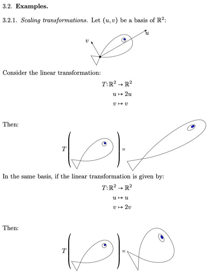
Definition (Scaling Transformation)

A linear transformation is a scaling transformation if there exists a basis of and scalars such that .

Note: later, we see that these transformations are formally called diagonalizable.

In scaling transformations, if , vectors are stretched along the corresponding basis vector and if , the vectors are shrunk along the corresponding basis vector. If = 0, it is a projection and if then there is no stretching. Finally, if , the vector is reflected along an axis perpendicular to the corresponding basis vector.

Linear Map

Proposition

Let be a basis of and let . Then,

Example: The derivative of polynomials is a linear transformation.

It is defined on its standard basis as .

Proof of linearity.

(a) Preserves addition:
(b) Preserves scalar multiplication

The so it is not surjective. However, if we redefine , the derivative is surjective. The derivative of the anti-derivative is the original function.
is also not injective since but . (This is why we need the "" when integrating)

Example: The integral/anti-derivative is a linear transformation.

It is defined on its standard basis as .

Proof of linearity.

(a) Preserves addition:
(b) Preserves scalar multiplication

Example: Notice that . So, is injective and is surjective. Note that .

Remark: The point of this section is to point out that it is only possible to have linear operators to be exclusively injective or surjective (i.e., XOR, not both) in infinite dimensional spaces such as and which are operators on .
In other words, in finite dimensional spaces, injective surjective bijective.

Projections

Definition (Projections)

A projection is a scaling transformation where all basis vectors are scaled by 0 or 1.
More formally, let be a vector space with a direct sum decomposition.
Then, every has a unique decomposition .
So, the projection onto along is defined as

So, .

Proposition

Projections are linear transformation

Proof.

(a) Preserves addition
Let .
and .

Since and , we have .
So, projections preserve addition.

(b) Preserves scalar multiplication
Let and .
Then, .

Therefore, projections preserve scalar multiplication.

Thus, projections are linear.

QED

Kernel and Image

Definition (Image)

The image (a.k.a. range) of is a subspace of the codomain and includes all vectors that have a corresponding vector in the domain.

Definition (Kernel)

The kernel (a.k.a. null space) of is a subspace of the domain where .

Proposition

surjective

Proof.

The definition of surjectivity, means that every is also so .
By the definition of image, .
So, in a surjective transformation, .

Proposition

injective

Proof.

(a) Show that injective

(a-i) Show that .

Trivial since kernel is a subspace.

(a-ii) Show that .

We know that
For contradiction, suppose there was another nonzero vector .
This is a contradiction since but violating injectivity.
Therefore, .

(b) Show that injective

Let such that .
Then, .
Since , .
Therefore, is injective.

Proposition (Homogeneous linear systems)

Let be a the matrix associated with the following linear transformation:

Then,

In other words, finding a basis of is algorithmically equivalent to for the solution set to a homogeneous system.

Proposition

Let be a vector space with basis and be a linear transformation. Then, the .

Proof.

(a)
Let . So, such that .
By taking coordinates, .
Then,

(b)
This is more or less the reverse of part (a).

Theorem (Rank-nullity)

Let be a linear transformation from vector space to , both finite dimensional. Then,

Matrix of a linear transformation

Proposition

Every linear transformation has an matrix in basis where the -th column of correspond to .

Furthermore, to generalize to , where is the basis for and is the basis for . Then, the matrix is rows and columns.

Example: Determine the matrix of in the standard basis . ( is the derivative defined in an earlier section)

Example: Determine the matrix of a rotation in the standard basis.

Definition (Composition)

If is a linear operator, the notation refers to -fold composition:

Main Isomorphism Theorem

The definition of isomorphism was previously introduced. Here we use some new notation to further explore isomorphism.

Let (phi) be an isomorphism between vector spaces and .
Since is bijective, then there exists an inverse where (psi).
Furthermore, we say that is isomorphic to , denoted , if there exists an isomorphism .

Theorem (Main isomorphism theorem)

Let be a vector space of dimension over a field .

Remark: Isomorphisms are very handy since we can solve many problems easily in and generalized to other abstract vector spaces by isomorphism.

Remark: Furthermore, to check if two spaces over a field are isomorphic, it is sufficient to check that .

Theorem

Let

Then, is an isomorphism if and only if is a basis of .

Proof.

(a) surjective

Firstly, we show surjective
surjective means that , . Therefore, and so .
Obviously, since the vectors are all in .

Secondly, we show that surjective.
Since , , we can express it as the sum for some values of ‘s. Then, . Since , we have found the corresponding such that , is surjective.

Therefore, the surjectivity if and only if spanning.

Another way to prove.
Let be the standard basis of . We also observe that since that standard basis of is 0 in all but the -th entry which picks out the .
surjective .

(b) injective is linearly independent.

injective .
So, .
Therefore, .
Therefore, is linearly independent.

Proposition

Let be an isomorphism and be vectors in . Then, .

Intuitively, it turns out that preserves linear relationships.

2. are linearly independent in are linearly independent in
3. is a basis of is a basis of

Rank Theorems

Corollary

If is a linear operator, the is an isomorphism, is injective and is surjective are equivalent.

It is obvious that isomorphism implies both injectivity and surjectivity by the definition of isomorphism.

Proof that injectivity implies surjectivity and isomorphism.

injective implies and .
By rank-nullity theorem, .
Since , .
Therefore, is surjective and furthermore is an isomorphism.

Proof that surjectivity implies injectivity and isomorphism.

surjective implies and .
By rank-nullity theorem, so .
Therefore, which implies injectivity and by extension isomorphism.

We know that (where elements in the kernel go to zero and elements that are outside the kernel don’t go to zero, there is not intersection since each value in the domain is mapped to only one element in the codomain). For the elements in , there exists an isomorphism with (i.e., ).

Definition (Rank)

Let be a matrix. The rank of , denoted is the dimension of the column space which we determine by counting the number of pivots in the REF.

Theorem (Rank-transpose)

The implication being that the column space and the row space of are equal which makes intuitive sense since they are the same pivots.

Change of Coordinates

Definition (Change of Basis Matrix)

Let be a vector space.
Then, define as a basis of and be linearly independent vectors in .

is the change of basis matrix from -coordinates to -coordinates.

To get an intuition for why indeed takes -coordinates to -coordinates, consider the following. The vector in -coordinates is . Then, when we apply the change of basis matrix , we get which pulls out the first column of which is . That is precisely is -coordinates. It is obvious that this pattern generalizes to and in fact all vectors in by linear properties.

Proposition

Let and be bases of . Define

to be the change of basis matrix from to -coordinates and

to be the change of basis matrix from to -coordinates.

Then, . Furthermore, in this case, the change of basis matrix is always invertible.

Intuitively, this makes sense. If we take a vector in -coordinates, change it to -coordinates and then change it back to -coordinates, it would be a surprise if we didn’t get back the original vector. Therefore, intuitively, .

Proof.

Let and be a basis of . We will also use an arbitrary vector .

Firstly, we can define the following isomorphism

By definition, the coordinates of in the -coordinates is .

Secondly, we can define another isomorphism

Again, by definition, the coordinates of in the -coordinates is

Therefore, the change of basis matrix from -coordinates to -coordinates, , can be decomposed as going from -coordinates to using and then going from to -coordinates using .

We can do a similar decomposition of change of basis from to -coordinates, .

To show

Remark (review from Math 133): Finding the inverse of matrices may be helpful. To do so, augment the matrix with the identity matrix and use Gaussian elimination to get RREF on the left side. The right side will be the inverse.

Definition (Change of Basis for a Linear Transformation)

Let be linear. Then, is the matrix of where is the basis of and is the basis of .

If we instead use a linear operator with both and being a basis of , then we get

Theorem (Change of basis formula)

Let , and . and are both bases of . Let denote the change of basis matrix from to coordinates and denote the change of basis matrix from to coordinates. These are related by the following formula:

Proof.

Since and , we can rearrange and get

This formula can be deduced intuitively. On the left-hand-side, takes vectors in -coordinates, and applies to them to get in -coordinates. On the right-hand-side, takes vectors from -coordinates to -coordinates. Then, takes vectors from -coordinates to in -coordinates. Finally, takes from -coordinates back to -coordinates. Overall, both sides achieve the same end goal, getting in coordinates. The only difference being that the left-hand-side does it directly while the right-hand-side does it indirectly via -coordinates.

Chapter 9: Diagonalization, Eigenvalues and Eigenvectors

Eigenvalues and Eigenvectors

Definition (Eigenvalue)

Let be a linear transformation. A scalar is an eigenvalue of if such that .

The equation means that and are collinear and scales by .

Definition (Eigenvector)

Given an eigenvalue for a linear transformation , a vector such that is called an eigenvector.

Definition (Eigenspace)

Let . The set of eigenvectors for a given is called the eigenspace of corresponding to the eigenvalue .

Proposition

Given .
If is not an eigenvalue, then .
If , then .

Proposition

The eigenspace is a subspace of .

Proposition

If , then .

Proof.

Let .
Since , .
Since , .

Therefore, . Since , and so .

Thus, and the inclusion going the other way is obvious since the intersection of subspaces is a subspace so it must contain the zero vector.

QED

Corollary

is scaling if and only if basis of eigenvectors if and only if such that .

Two examples of linear transformation that are not scaling are rotations and shearing. For rotations, the exceptions are when or which for shear with matrix , the vectors on the -axis are scaled by (i.e., unaffected) while other vectors are not scaling.

Proposition

Let be the matrix associated with a linear transformation .

Then, is a scaling transformation is diagonalizable.

Proof.
Let be a basis of eigenvectors of (i.e., the ‘s are eigenvectors and they form a basis). This is possible by definition of scaling.
To write , we compute in the -coordinates. Since (and using the -coordinates of the where all zero except the corresponding entry with one), we get

Let be the diagonal matrix. Then, we use the change of basis matrices between and -coordinates for and .
Then overall, we get .

How to diagonalize

Let . The following 2 steps are required to diagonalize.

1. Find the eigenvalues of .
2. Find the eigenspaces for each .

which can be solved by the homogeneous system .

Definition (Geometric multiplicity)

Let . Then

is the geometric multiplicity of eigenvalue for matrix .

Proposition

is diagonalizable

Corollary

If we have distinct eigenvalues, then is always diagonalizable since the minimum is 1 for any eigenvalue.

Theorem

The eigenvalues of are the roots of the characteristic polynomial

If we use polynomial factorization to get the following form

where the eigenvalues ‘s are pairwise distinct, then is diagonalizable.

Remark: By the fundamental theorem of algebra, we know that it is always possible to factorize over the field but not always over the field the implication that over only some matrices are diagonalizable while over all matrices are diagonalizable.

Summary: Given , find and . To find , we first find all of the eigenvalues

Polynomials of matrices

Definition (Powers of Matrices)

Let .

Theorem

Suppose is diagonalizable. Then, is also diagonalizable.

The powers of diagonal matrices are easy to compute since each entry is just raised to the -th power (this is not true in general, only diagonal matrices).

This can be generalized to apply to polynomials of matrices.

Then, for the diagonal matrix, just apply to each entry (once again this is specific to diagonal matrices and not broadly applicable to general matrices).

Theorem (Cayley-Hamilton)

For an arbitrary square matrix , the characteristic polynomial satisfies .

Chapter 7: Inner Product Spaces and Orthogonality