For fast on-demand sampling from large categorical distributions, pip install categorical, and check out the API examples below, and the benchmark against numpy. Beating Dynamic Time Warp for Fast Sequence Alignment

The Problem: String Edit Distance

Disamgiguation note. There are a few related problems that are easily confused. Pairwise sequence alignment, which is the topic of this post, is the problem of finding the best alignment between two sequences. In string matching with k differences the goal is to find all occurences of one string within another, affording k edits. In general, solutions to one problem don't directly yield solutions to the other, and vice versa.

Consider the spelling of the words brexit and elite. There is a certain sense in which they are more similar to eachother than either is to the word covfefe. For one, brexit and elite have three letters in common. Not only that, those letters are in the same order.

We can formalize the notion of string similarity by asking: “how many edits do we need to make to turn one string into the other?” We let an “edit” be one of the following:

• Delete a character.
• Insert a character.
• Change one character into another.

Turning brexit into elite would look like this (the pipe “|” shows where an edit will happen):

0. |brexit
   
1. b|rexit
   
2. bre|xit
   
3. brelit|
   
4. brelite
   

Minimum Edit Distance \(\iff\) Sequence Alignment

So in one sense, we can say that brexit has distance 4 from elite. We can depict the two strings and the needed edits concicely by aligning preserved characters:

brexit·
**|*||*
··elite

Preserved letters are connected by |’s. Substitutions, ininsertions, and deletions are indicated by *’s, and you can tell them appart based on the identities of the original (upper) and new (lower) character.

As this diagram suggests, finding an alignment that matches as many characters as possible will allow you to conserve as many edits as possible. So finding the best string alignment (allowing for gaps) is really the same problem as finding the minimal sequence of edits to convert one string into the other.

For this idea to work as a measure of string (dis)similarity or distance, we need a way to work out the minimum number of edits between any two strings \(s\) and \(t\). If you've never seen the solution before, writing an algorithm that finds this minimum in a reasonable amount of time can be pretty devilish. Individual edit decisions potentially involve long-range tradeoffs, and there are many possible sequences of edits that take \(s\) to \(t\).

Generality

When comparing time-series, the problem is often set up to exclude deletion and insertion, but allow multiple elements of one sequence to be identified with an element of the other. In that case \(\delta\) is more aptly described as an elementwise (dis)similarity function, rather than an edit cost. This problem doesn't only involve strings. Any discrete sequence—video frames, audio samples, nucleotide bases, keystrokes, etc.—can be analyzed in this way. And to step into this more general stance, it might make sense to think of some edits as more significant than others. So, we posit that every edit comes with a cost, and the cost depends on what characters are involved in the edit:

• Delete element \(c\) at a cost of \(\delta(c,\cdot)\).
• Insert element \(c\) at a cost of \(\delta(\cdot,c)\).
• Replace element \(c\) with element \(d\) at a cost of \(\delta(c,d)\).

Notice how we can think of insertions and deletions as a substitution involving the empty character “\(\cdot\)”.

We will stipulate a few constraints on \(\delta\), as is typical:

1. edits can't have a negative cost:
   \[\delta \geq 0.\]
2. the triangle inequality holds:
   \[\delta(c,d) \leq \delta(c,e) + \delta(e,d).\]
3. there is no cost to leave a character unchanged. \[\delta(c,c)=0, \quad \forall c \in \Sigma,\] Where \(\Sigma\) is the alphabet of characters.

The following must hold for cost function \(\delta(c,d)\), defined over pairs of characters \(c,d\) from alphabet \(\Sigma\) (which includes the empty character): \[ \begin{equation} \begin{split} \forall c,d \in \Sigma: & \quad \delta(c,d) = \frac{p}{q},\\ & \quad \text{where} \quad p,q \in \Bbb{Q},\\ & \quad \text{and} \quad \frac{\delta_\text{max}}{q} \ll n, \end{split} \end{equation} \]

There is one other constraint on \(\delta\) that is needed by a method I'll introduce later. The costs should be integers, and the largest cost (after dividing all costs by their greatest common factor), shouldn't be too big; say less that 1024. We'll unpack the need for this constraint later. See the margin for some more details.

For our examples, we'll fix \(\delta\) to be 1 for all insertions and deletions, and 2 for all substitutions: \[ \delta(a,b) = \begin{cases} 0 & \text{if } a = b \\ 1 & \text{if } a = \cdot \text{ or } b = \cdot \\ 2 & \text{otherwise } \end{cases} \] Notice that a substitution is like a deletion followed by an insertion, so it makes sense for them to cost twice as much. In any case, the reasoning that follows applies to any \(\delta\) that meets the stated constraints.

A Linear Approach

Let's get a feel for why this is a tricky problem. Imagine an algorithm that proceeds through the two strings, a few characters at a time, based on local information. Let's say the algorithm solves windows of three characters at a time.

We set the algorithm to work on on two strings, \(s=\)"abcdba" and \(t=\)"adbaaa". First the algorithm aligns the first three characters, this gives us:

   a·bc
   |*|*
   adb·

Now, continuing on, if the algorithm does it's best to align the next three characters,

             a
             aabdba                      abcdba
   we get    |*|***|     but we want     |**|||    .
             adb·aaa                     a··dba

a-hix---hijk
a-hijk--h--

 abcbc

This example shows how later parts of the string can make initially good decisions turn out to be wrong. We can't just proceed making the best decision possible given the strings so far. It's nothing special with a window of 3 characters either. It's just the case that the best alignment of n characters isn't necessarily part of the best alignment of n+1 characters.

Imagine that we try to write a program that will proceed through the pair of strings, and write edits, one a time. You can imagine a machine with two stacks (containing the characters). The machine does a sequence of inserts, edits, and deletes, and corespondingly a character is popped of one or both stacks. Can such a program determine the best alignment merely by looking at the top of each stack, in one pass?

It's easy to construct a couple examples to show that such a program can't solve the problem. First, let's suppose that we want to align axbc with aybc. We can animate the single linear-pass machine like this:

   a·bc
   |*|*
   adb·

             a·bcdba                     abcdba
   we get    |*|***|     but we want     |**|||    .
             adb·aaa                     a··dba

Basically, we have to pay for inserting the x and deleting the c. This alignment involves matching the b’s.

Even in this simple example, you can start to see how things can get complicated. Let's imagine, for a moment, processing the strings, one character at a time, and making editing decisions. I'll let a ▒ represent the cursor.

Clearly, at this moment, since a matches a, we should not do an edit, and we should accept the zero-cost for a match. That leaves us in the following state:

Here we may want to make an edit. We could substitute b\(\to\)x. We could delete b\(\to\cdot\). Or we could insert \(\cdot\to\)x. Now, looking ahead, it's obvious that we should “save” the b by inserting \(\cdot\to\)x, so that in the next moment, we can match up the b’s. So we get this:

The point is to figure out how to handle the x and b, we had to look ahead. Think about it: it's not hard to construct cases where you'd need to look arbitrarily far ahead. The trouble is that you don't have enough information at a given point in the string to the best decision.

Dynamic Time Warping

This is a “dynamic program” that appears to have been discovered independantly by many people. The algorithm works by first solving the problem on prefixes of \(s\) and \(t\). In other words, it finds the minimum edit distance between the first \(i\) elements of \(s\) and the first \(j\) elements of \(t\).

First, we solve the problem for \(i,j=1\), in other words, we find the edit distance between a and a, which is obviously 0. Next, we solve when \((i,j)=(2,1)\), i.e. for (ab, a). Easy again, it's 1, since we clearly need to delete the b. Similarly, solving for \((i,j)=(1,2)\), we have (a,ax), and the solution is to insert an x (we take the perspective of editing \(s\), but you could also think of this as deleting x from \(t\)).

So far so good, but the magic of dynamic programming starts become visible itself when you look at \((s,t)=(\)ab, ax\()\). Although it's fairly obvious that the answer will be 2, we can write the distance \(D(\text{ab},\text{ax})\) in terms of subproblems : \[ D(\text{ab},\text{ax}) = \min \begin{cases} \delta(\text{b}, \text{x}) + D(\text{a},\text{a}) \\ \delta(\cdot, \text{x}) + D(\text{ab},\text{a}) \\ \delta(\text{b}, \cdot) + D(\text{a},\text{ax}) \\ \end{cases} \] The three lines under the minimum operator can be respectively phrased in plain English as:

• the cost to substitute x for b, plus the minimum edit cost between a and a
• the cost of deleting b, plus the edit cost between a and ax; or
• the cost of inserting x, plus the edit cost between ab and a

It might seem unnecessary, but notice that we can always use that decomposition to express one minimum edit distance problem in terms of smaller ones.

Stating it generally, the minimum edit distance between \(s\) and \(t\) is given by the smallest among:

• the cost to substitute \(t_m\) for \(s_n\) (usually 0 if \(s_n = t_m\)) plus the edit cost between \(s_{-1}\) and \(t_{-1}\);
• the cost of deleting \(s_n\), plus the edit cost between \(s_{-1}\) and all of \(t\); or
• the cost of inserting \(t_m\) onto the end of \(s\), plus the edit cost between \(s\) and \(t_{-1}\)

Where \(s_{-n}\) denotes \(s\) without it's last character, which is itself denoted by \(s_n\). The true minimum cost must be given by one of these cases, and each of them is expressed in terms of solutions to smaller problems. To put it more mathly, \[ D(s, t) = \min \begin{cases} \delta(s_n, t_m) + D(s_{-n}s_{n}, t_{-m}t_{m}) \\ \delta(\cdot, t_m) + D(s, t_{-m}t_{m}) \\ \delta(s_n, \cdot) + D(s_{-n}s_{n}, t) \\ \end{cases}. \]

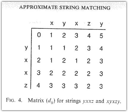
Returning to the example of finding the minimum edit distance between abc and axb, we can depict the necessary calculations for our example in a trellace:

Each cell holds the minimum edit cost when matching prefixes up to and including the letters heading the cell’s row and column. Moving down corresponds to deletion; moving right corresponds to insertion; and moving diagonally, down and to the right, corresponds to substitution (or to the alignment of like characters, typically at no cost). The first cell is at the top-left, and it corresponds to the null subproblem—the edit distance between the empty string and itself. Calculation proceeds down and to the right, until it reaches the cell representing the edit distance between the full strings \(s\) and \(t\), shown above with a heavy border.

Dynamic Time Warping is Too Slow

All the combinations of prefixes of the input sequences, for all prefix lengths, have to be considered. If the lengths of the sequences are \(m\) and \(n\), then dynamic time warping takes \(O(nm)\) time. This is too slow: on today's hardware, it is an impractical approach to align the characters in two news-article-lengthed texts.

Wasting Time on Bad Subproblems

If you dig into the details of the dynamic time warping algorithm, you will notice that it wastes a lot of time looking at subproblems that usually don't end up contributing to the final solution. For example, it solve a subproblem in which first character of one sequence against the entirety of the other sequence. But such a solution only comes into play if the two sequences have almost no matching characters at all.

So, why not start by checking if the sequences can be matched with \(k\) or fewer differences first? Any subproblem that can't participate in such a solution can be forgone, at least until we discover that no alignments are possible given \(k\) or fewer edits.

Diagonal Banding Approach

In 1985, Esko Ukkonen proposed such an approach. In addition to the strings \(s\) and \(t\), Ukkonen’s algorithm takes in the maximum edit distance \(k\). The algorithm either outputs the distance, or fails if no alignment (sequence of edits) could be having a cost of at most \(k\).

As a result, the running time for Ukkonen's algorithm is \(O(kn)\), assuming \(n\) is the lesser of \(m\) and \(n\).

If there are not too many errors in the text, this is way faster. For example, in my application, I am usually trying to reconcile two very similar versions of a text. Often the texts will have been processed by algorithms or maually by people, to add grammatical or semantic annotations. In the process, the texts might be altered, like squashing everything into ASCII, or normalizing opening quotes as `` and closing quotes as ''. In those situations, I don't expect there to be too many differences between the two texts.

We Can Still Do Better

While Ukkonen's algorithm can give a major speedup, it requires that you bound the number of errors ahead of time. I don't generally know how many errors there will be. But, if I set \(k\) too large, I don't get the speedup that I want. Of course, you could easily write a program that re-runs Ukkonen's aforementioned algorithm with a larger value for \(k\) when it fails, which Ukkonen proposed.

That seems ineligant to me, and hints that there might be a progressive algorithm that explores alignments with gradually higher cost, efficiently using partial solutions for alignments with lower costs.

I set on this problem, and found that you can write an \(O(kn)\) variation that doesn't require the specification of \(k\) ahead of time

Use Breadth First Search to Evaluate Subproblems

The key innovation is that the algorithm is strategic about the order in which to evaluate subproblems. As the algorithm proceeds through subproblems, it keeps track of the best possible score that could be obtained from a global solution involving that subproblem. Using this information, it proceeds to solve those subproblems that contribute to the best possible global solution first, and only move on to subproblems that are part of less optimal global solutions later.

When the algorithm evaluates the score for maching prefixes of lengths \(i\) and \(j\), it also calculates the minimum cost that could come from continuing the matching from that point until the end. That is, for each subproblem, it calculates cost and a best case scenario cost for completing the match from that point onward.

A few insights are needed to make this actually a better approach.

First of all, finding the best case scenario cost is easy: given some prefix match, if the length of the remainders of the sequences are not equal, then we will need to pay for a number of insertions or deletions equal to the difference in their lengths. We therefore add onto the current cost a cost equal to the number of insertions or deletions times the minimum insertion or deletion cost.

And second, we proceed through the subproblems using a breadth-first-search approach, always expanding the search through subproblems that have the as-yet-lowest best case scenario cost.

To understand how we might apply a breadth first search through subproblems, we first need to understand how the subproblems can be seen as forming a graph.

In the usual dynamic time warping algorithm, we lay out the subproblems in a grid as depicted below. In solving the \((i,j)^\text{th}\) subproblem, we need to consider the solutions to problems that come “before” it. That means having the solution already to \((i,j)\), \((i-1,j)\), and \((i-1,j-1)\). In this way \((i,j)\) depends on its neightbours above and to the left of it.

If we consider each subproblem as a node, and draw a directed edge from each subproblem towards those on whose value it depends, we obtain a the dependency graph.

However, we want to consider a slightly different graph, in which all of the edges of the dependency graph have been reversed. In other words, we draw edges to nodes that can depend on a source node, as opposed to drawing an edge from the source node to nodes it depends on.

We begin evaluating subproblems starting from \((0,0)\), and in a way reminiscent of Dijstra's algorithm, we continually expand our search out from the subproblem having the best best-case-scenario score.

If we are clever enough to pursue a path through this graph in breadth-first-search first order, then every time we calculate the next subproblem, we can assume that we the neighboring subproblem from which we came contributes the best score. Since, if that were not the case, we must not be following the breadth-first-search order.

, can yield a score of \(k\), and only moving on to others by \( We can think of the \((i,j)^\text{th}\) subproblem as connected to its neighboring subproblems, \((i+1, j)\), \((i,j+1)\), and \((i+1,j+1)\), in the sense that it provides information to each of these neighboring subproblems, but only if no other neighbor to these subproblems is better than \(i,j)\).

For any given value of \(k\), there are certain partial matches which cannot yield a solution whose score is less than \(k\). You’ve probably done this many times: you’re writing a program that needs stochasticity—with some probability \(p_A\), event \(A\) should occur, otherwise \(B\) should occur. You sample a pseudorandom number from \([0,1]\), and if that number is smaller than \(p_A\) you execute event \(A\), and otherwise \(B\). And if you’ve got three outcomes, or five or twenty, this generalizes nicely: you just divide up the interval \([0,1]\) into subintervals, or “bins”, whose sizes correspond to the the desired probabilities, sample your pseudorandom number, and then test which bin it falls in.

But the catch is that this requires scanning through the interval to see which bin the pseudorandom fell into. You end up with something like this:

import random

picker = random.uniform()	# a pseudorandom in [0,1]
if picker < p_1:
	outcome = 1
elif picker < p_2:
	outcome = 2
elif picker < p_3:
	outcome = 3
...
else:
	outcome = k

“On the order of \(k\) tests”: if you get lucky, and most of the interval is covered by a small number of outcomes, then you might do better than \(O(k)\). But that only works for distributions having particular properties. You could write it more compactly in a loop, but it doesn’t change the fact that you’ll need to do on the order of \(k\) tests. And if \(k\) is large, and you need to draw a lot of samples, this isn’t good!

I ran into the need to draw samples from a categorical distribution with larege support when I was implementing word2vec. In the training algorithm, you need to sample an English word randomly according to the frequency that words appear in a large corpus. Depending on how you count, there are hundreds of thousands of English words, or millions. Repetitively testing so many interval endpoints every time you sample a word is just too slow. But, there is a better way.

A Better Way: the Alias Method

It turns out that you can draw a sample according to your target categorical distribution in constant time. The approach builds off the fact that, if you had wanted to choose one of \(k\) equally likely possibilities, then sampling in constant time would be simple: Equivalently, you could call random.randint(), but for illustrative purposes, I’m assuming we’re building off a pseudorandom primitive that gives uniform samples from [0,1].

outcome = int(random.uniform() * k)

The trick in the alias method is to convert our sampling problem, in which outcomes have varied probabilities, into something more like sampling from a uniform distribution. To do that, we’re going to create alias-outcomes, each of which actually stands for a combination of two of our original outcomes. Then, we’ll have a way of figuring out which of our original outcomes should be produced from the alias-outcome in such a way that samples are generated according to the original distribution.

Setting up Alias-Outcomes

First, notice that, if our original distribution had been uniform, then each outcome would have probability \(1/k\). Since our distribution isn’t uniform, it means that some outcomes have more than \(1/k\) probability, and some have less. With that in mind, we can imagine constructing alias-outcomes by combining one of the outcomes having less than \(1/k\) with a small “donation” of some probability mass from one of the higher-probability outcomes, topping up the total probability for that alias outcome to \(1/k\). Then we use the leftover mass from the higher-probability outcome in constructing another alias-outcome. We can obtain a set of \(k\) alias-outcomes in this way, each of which was made by a donation of mass from one or two of our original outcomes (Figure 1):

When building the alias outcomes, we need to keep track of which original outcomes contribute to which alias-outcomes, and how much. We can store this information in arrays of length \(k\), and it will take us \(O(k)\) to set up the arrays. But, we only need to do that once, and then, sampling can be done quickly as follows. First, we sample one of the alias-outcomes according to the uniform probability. This is fast because they are uniformly distributed. Then, we look up which original outcomes were used to make that alias, and how much each contributed. Since only two original outcomes makeup each alias, we can sample one of these using the “simple way” we saw in the opening paragraph. So, sampling from the original distribution can be done in constant time, by drawing two samples from \(U(0,1)\).

I find myself having to sample from categorical distributions fairly often. Numpy supports that with numpy.random.choice(), but depending on your usecase, it can be slow. The problem with numpy.random.choice() is that it seems to rebuild the sampler every time (although I don’t know how it’s implemented). If you know ahead of time that you want, say one million samples, then you can request them all at once, and this is fast. But if you can't or don't want to get your samples ahead of time, then numpy’s implementation is quite slow. Clearly they have an efficient sampler under the hood, so it seems like just a lapse in the API that the underlying sampler isn't exposed to the user.

Because of this, I packaged up an implementation called categorical that uses the alias method and provides the user with a sampler instance that can produce samples on demand faster than individual calls to numpy.random.choice(). If you know ahead of time how many samples you need, numpy’s implementation will serve you better. But if you don’t want to or can’t generate all the samples ahead of time, then my implementation will give you fast on-demand samples. You can include categorical in your projects with a simple pip install, see below.

categorical Installation and Usage

Install from pip: pip install categorical

Let’s generate a probability distribution to get us started. First, sample a bunch of random numbers to determine probability “scores”.

>>> from random import random
>>> k = 10**6
>>> scores = [random() for i in range(k)]
>>> total = sum(scores)
>>> probabilities = [s / total for s in scores]

We've normalized the scores to sum to 1, i.e. make them into proper probabilities, but actually the categorical sampler will do that for us, so it’s not necessary:

>>> from categorical import Categorical as C
>>> my_sampler = C(scores)
>>> print my_sampler.sample()
487702

The value 487702 above means that the sampler yielded the outcome corresponding to the 487703^rd outcome, as listed in the probability-scores provided to the constructor (outcomes are zero-indexed of course). Since we hadn’t normalized the probability scores in advance, we can ask the sampler what the probability of sampling that outcome was:

>>> my_sampler.get_probability(487702)
5.3028349767480922e-07

Pretty small indeed!

As a bonus, you can provide a shape parameter when calling sample, and get back a numpy array, having the specified shape, filled with independent samples:

>>> my_sampler.sample((3,4), dtype='int32')
array([[719441, 321772, 741180,  93447],
       [652309, 472908,  40968, 422349],
       [993621, 652970, 720311,  79800]])

Benchmarking Against numpy

Comparing to numpy, assuming we draw 1000 samples individually:

>>> from numpy.random import choice
>>> import time
>>> 
>>> def time_numpy():
>>> 	start = time.time()
>>> 	for i in range(1000):
>>> 		choice(k, p=probabilities)
>>> 	print time.time() - start
>>> 
>>> def time_my_alias():
>>> 	start = time.time()
>>> 	for i in range(1000):
>>> 		my_sampler.sample()
>>> 	print time.time() - start
>>> 
>>> time_numpy()
31.0555009842
>>> time_my_alias()
0.0127031803131

If instead, you draw your samples upfront, numpy might be faster, depending on how many samples you want. At around 10,000 samples taken in batch, numpy starts to get faster:

>>> def time_numpy():
>>>     start = time.time()
>>> 	choice(k, size=(10000,), p=probabilities)
>>> 	print time.time() - start
>>> 
>>> def time_my_alias():
>>>     start = time.time()
>>>     my_sampler.sample(shape=(10000,))
>>>     print time.time() - start
>>>
>>> time_numpy()
0.107708930969
>>> time_my_alias()
0.117538928986

So, if you are drawing more than 10,000 samples at a time, numpy will be faster, whereas if you are sampling fewer than that (especially if you do so repeatedly), then categorical will be faster.